NYC Community Clustering

New York has a rich tapestry of ever-changing neighborhoods. These regions act as a lens to help us describe the city’s communities, and because of this people often have strong opinions on how they should be defined. But neighborhoods don’t tell the full story, and real communities aren’t always confined to these named boundaries. Understanding how people group together, independent of what we call an area, is a crucial part of learning the values and needs of a city at the local level.

In this project, I study these communities through an alternate lens: demographic and economic similarities. I harness machine learning methods to spatially cluster the city into geographically compact regions of similar people and households. Investigating how these clusters differ from the usual neighborhood boundaries reveals some interesting insights into the city’s human geography. If that sounds interesting to you, read on!

Gathering data

I pulled data from the 2020 US Census Demographic Profile and the 2023 5-year American Community Survey at the Census tract level. Using a combination of PCA, linear and nonlinear regression analysis, and spatial autocorrelation checks, I chose 11 largely independent features with interesting spatial structure. They cover a wide gamut of information:

• (4) Race and nationality.
  • Fractional populations of Hispanic, non-Hispanic white, non-Hispanic black, and other (this is three independent features because the fractions sum to 1).
  • The fraction of foreign-born residents.
• (2) Age.
  • Median age and fractional working age population (between 18-64).
• (2) Household type and socioeconomic status.
  • Median household income.
  • The fraction of household owners living with their spouse.
• (3) Urbanization.
  • Population density.
  • The amount of large (20+ unit) apartment buildings and the fraction of people who commute to work by walking.

Using a spatially aware clustering algorithm

When clustering geographies into local regions, we actually need to balance two competing desires: to group demographically similar Census tracts together (those with “feature similarity”) and to create geographically compact clusters. Common methods like K-Means only consider the former, leading them to group spatially distant regions together:

Each color represents one cluster. See how demographically similar parts of Staten Island and Queens are grouped together, ignoring the local nature of communities: that's not what we're looking for.

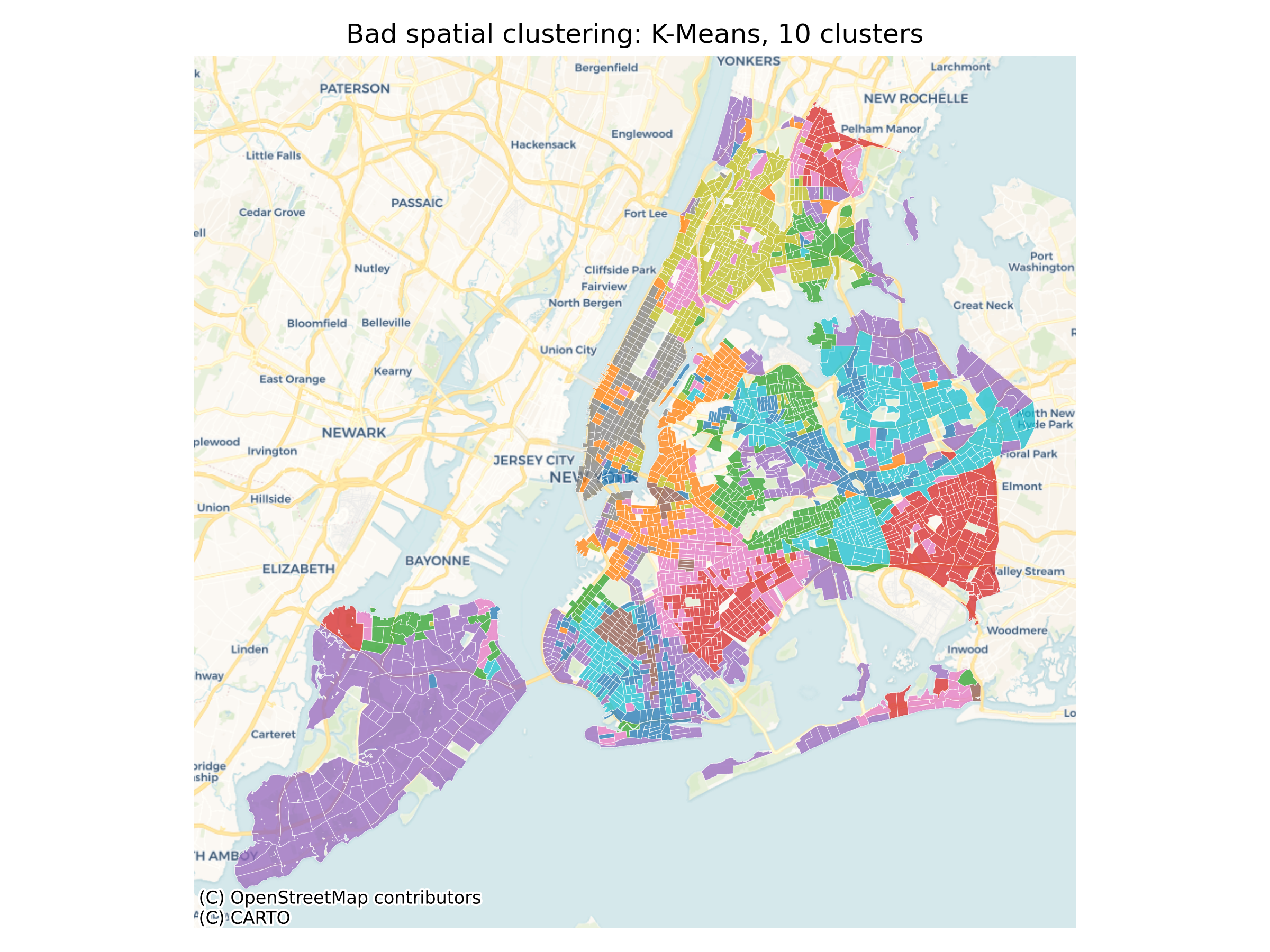
Instead, I used an algorithm belonging to a family of methods called REDCAP¹, which explicitly require clusters to be contiguous. This algorithm performed the best on a combination of metrics, chosen to value both geographic compactness and feature similarity:

• The Polsby-Popper score (evaluates geographic compactness)
• The Davies-Bouldin score (evaluates feature similarity)
• The “path” silhouette score² (combination of both).
  • I actually modified the metric to fix some perceived issues (documented in the project notebooks for anyone who’s curious).

Results

Check out the results of my clustering algorithm in this interactive map! You can visualize demographic features like race, age, and income for three clusterings with different numbers of clusters (low, medium, and high).

Using my custom evaluation metrics, these clusters stack up well against pre-defined neighborhood boundaries. I compared against 2017 Zillow neighborhood boundaries (publicly shared here), as well as the city’s own Neighborhood Tabulation Areas (NTAs). All three clusterings score at least:

• 30% lower on the Davies-Bouldin score than the NTAs and 20% lower than the Zillow boundaries (lower is better)
• 15% higher on my modified path silhouette score than the NTAs and 34% higher than the Zillow boundaries (higher is better).

What can we learn from this?

There’s a ton of fascinating structure here, and I dig into many details in the project repository. Here, I’ll highlight two examples.

Gentrification Boundaries in Williamsburg

Williamsburg has experienced rapid demographic change in recent years. In the present day, these dynamics are reflected by the existence of three distinct clusters in the neighborhood:

Comparing demographic clusters in Williamsburg. Notice how cluster 29 (blue) is consistently whiter and wealthier than cluster 23 (orange).

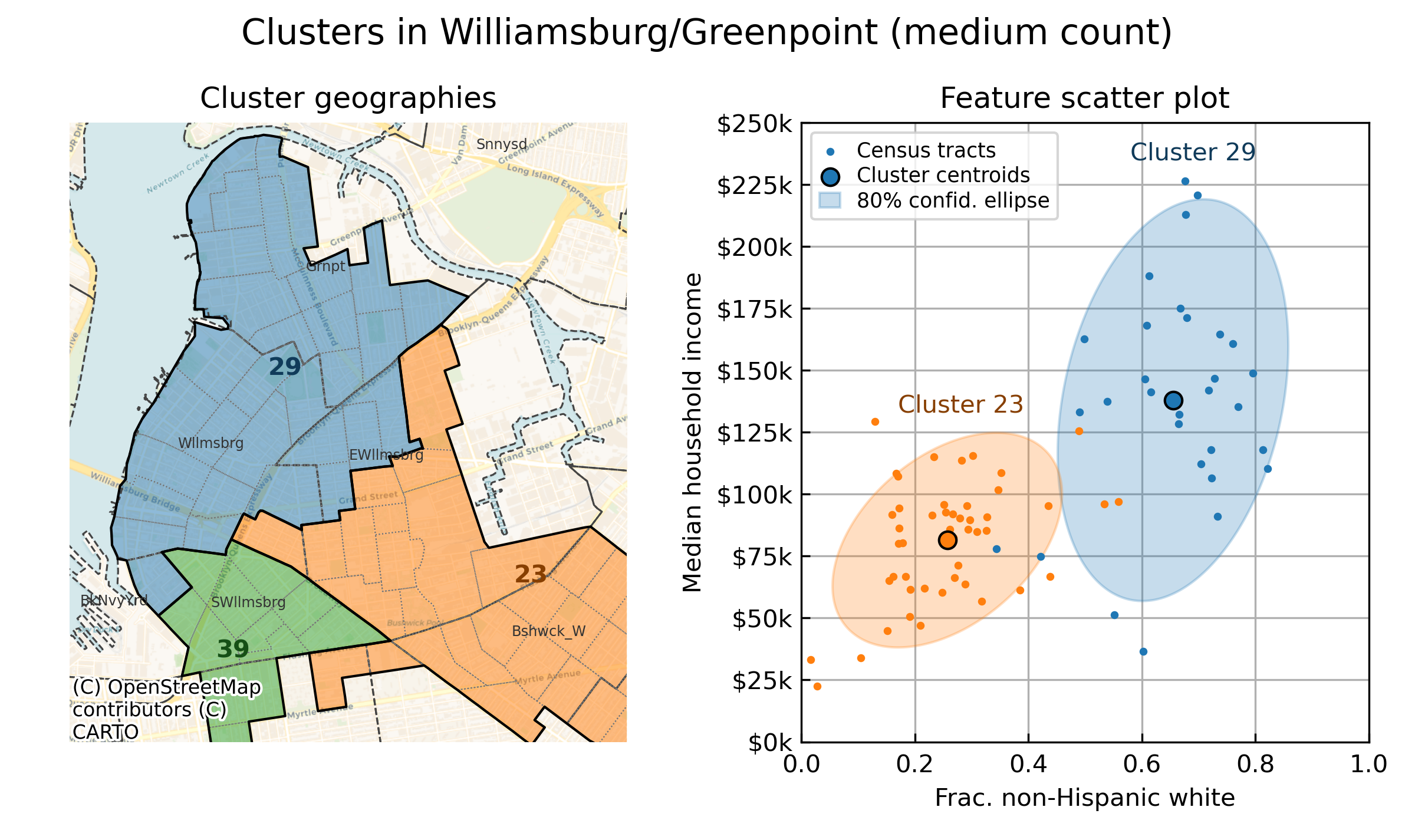
The green cluster represents the Hasidic Jewish community in South Williamsburg. It’s strongly internally homogeneous, and the algorithm readily detects its distinctively high fraction of married households and hyperlocal commuters who walk to work.

Less obvious at a glance is the boundary between the blue and orange clusters, which lies somewhere in eastern Williamsburg. Diving into feature space with the scatter plot reveals the reason: two classic gentrification markers, median household income and the fractional population of white residents, undergo a transition in this area that separate central Williamsburg and Greenpoint from eastern Williamsburg and Bushwick. The cluster boundaries give us a sense of roughly how far “peak” gentrification extends in the neighborhood.

Housing Zone Demographics in Forest Hills

The housing stock of an area can have a strong impact on its demographics. Take the Rego Park and Forest Hills area as an example: here, my clustering algorithm detects a natural boundary splitting both of these neighborhoods down the middle:

Comparing two demographic clusters in Forest Hills and Rego Park. In this area, the fraction of married households is strongly negatively correlated with the fraction of 20+ unit apartment building.

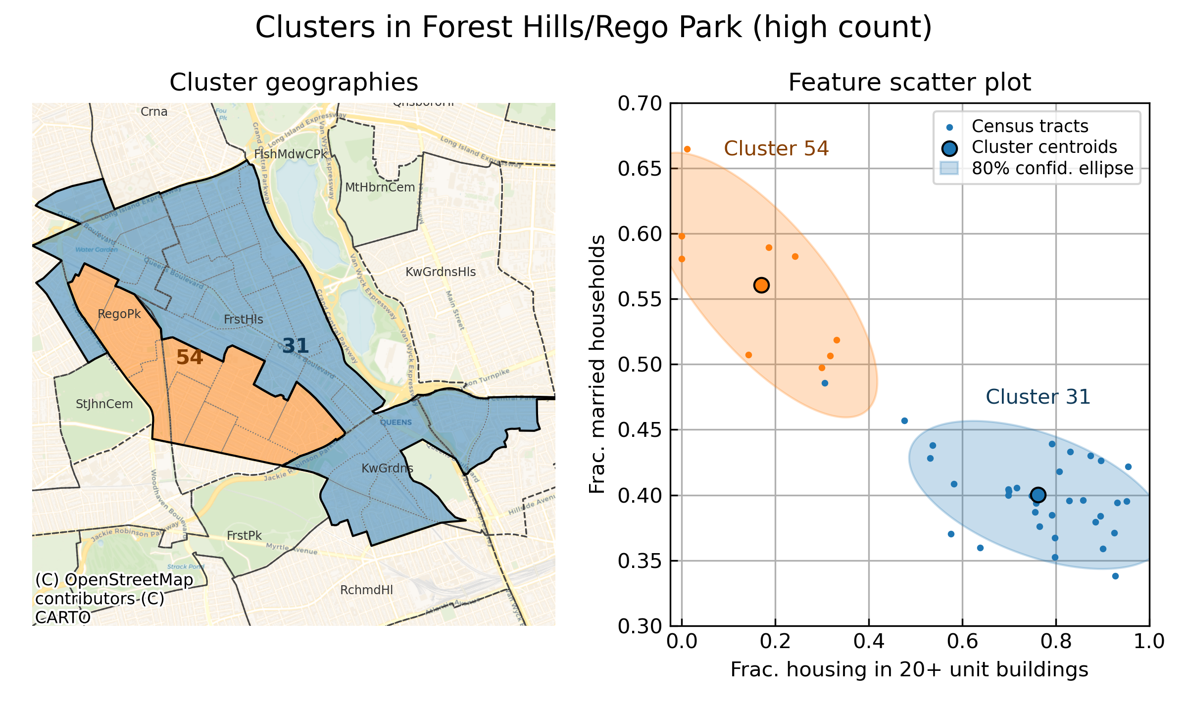
This boundary, roughly following the LIRR line south of Queens Boulevard, separates Census tracts with high density housing to the north (blue cluster) from lower density housing to the south (orange cluster), consistent with the different housing zones in the region. Feature space shows that married households consistently prefer living in the orange cluster, indicating a community with a more suburban feel compared with the transit corridor in the north.

The takeaway: these two communities are defined not by neighbhorhood boundaries but rather by transit geography and housing policy, and my clustering algorithm can detect them!

Conclusion

This project taught me that, given the right features and clustering methodology, we can unveil real demographic structure that sheds light on the city’s geography. Looking forward, these clusters can act as natural filters for analyzing other data (like the American Community Survey) to teach us a ton of information about these local demographic communities—information like educational attainment, type of employment, insurance coverage, and more. You could also look for needs or inequities at the community level. For example: are some demographic communities food or transit deserts, even if their neighbhorhoods are well-served in aggregate? Are there regions with many elderly but poor access to nearby healthcare?

For now, though, this ends my exploration. If you want to dive into the data yourself, check out my GitHub project here!

---

References

1. Guo, D. (2008). Regionalization with dynamically constrained agglomerative clustering and partitioning (REDCAP). International Journal of Geographical Information Science.
2. Wolf, L. J., Knaap, E., and Rey, S. (2019). Geosilhouettes: Geographical measures of cluster fit. Environment and Planning B: Urban Analytics and City Science.